Camera
Users can choose from various display and capture sizes, and adjust live image settings such as white balance, brightness, contrast, hue, and saturation. Once configured, the image can be captured and saved to the designated folder for further analysis.

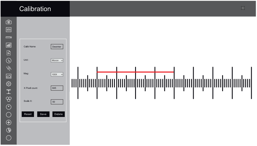
Calibration
Calibration must be carried out for all microscope objectives where a digital camera is installed. It should only be performed after all hardware components are securely in place. If any part is readjusted or replaced, recalibration is required.
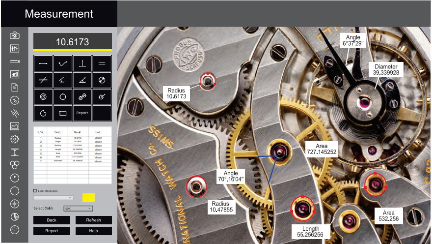
Measurement
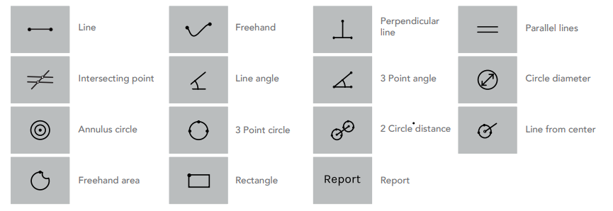
The Measurement module allows users to take measurements by manually drawing lines on traces, shapes, or object outlines. These measurements can be recorded in the results worksheet, where they can be saved to a file, printed, or exported to a spreadsheet for further analysis or statistical evaluation.
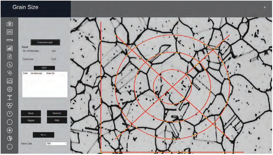
Grain Size
This module performs fast, objective, and repeatable grain size analysis according to industrial standards, supporting evaluation of ferritic and austenitic grain structures in steel. It follows international methods including ASTM E112, E93, and E1181.
A comprehensive range of analysis techniques is available:
- Lineal Intercept Method
- Abrams Three-Circle Method
- Snyder & Graft Method
- Comparison Method
- Random Intercept Method
- Manual Grain Size
The built-in wizard calculates the grain number, mean grain area, and mean intercept length at high speed based on the selected method.

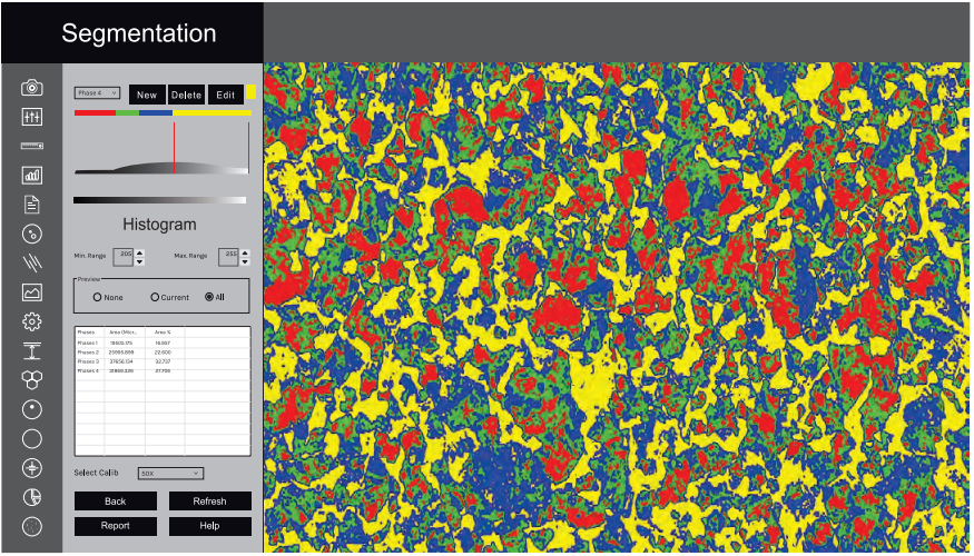
Segmentation
Segmentation is a technique used to partition an image based on the intensity or grayscale values of its components. Phases within the image are detected and their areas calculated according to these grayscale values. Users can delineate phases directly from the histogram, which enhances accuracy in phase identification.
Multiple phases are represented with color overlays and can be displayed simultaneously within the same field of view. The resulting segmented images and data are saved to clearly distinguish each phase. Prior to segmentation, filters such as Despeckle and Smoothing can be applied to improve image quality.
HISTOGRAM
When the Segmentation module is launched, a grayscale histogram is automatically generated. The X-axis shows intensity values ranging from 0 to 255, while the Y-axis displays the number of pixels corresponding to each intensity level. The system supports industry-standard analysis.
Users can define up to ten threshold levels to identify and label different material phases. Each phase is represented by a specific color between the selected thresholds.
- INTENSITY
The intensity range of the active phase is continuously shown in the dialog box, helping users monitor and adjust settings in real time. - SELECTED PHASE
This function allows users to click within the histogram to determine the percentage area of a specific intensity range. To ensure accurate results, any prior selections must be cleared, and the preview mode should be set to "None."
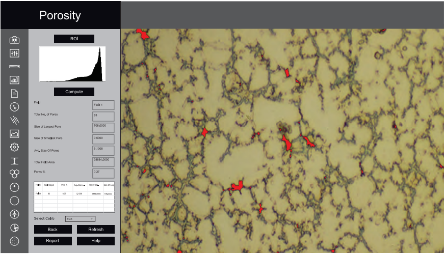
Porosity
Pores are relatively easy to detect due to their contrast with the surrounding material. This module automatically identifies and measures porosity in accordance with ASTM B276 standards. Thresholding is performed using grayscale techniques, and the dark phase representing porosity is highlighted in red bitplanes.
The system automatically counts the total number of pores and reports their size distribution, including the minimum and maximum pore sizes as a percentage. The entire process is fully automated, ensuring fast and consistent results.

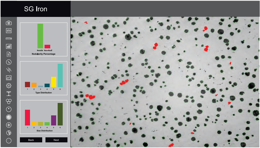
Ductile Iron/Nodularity
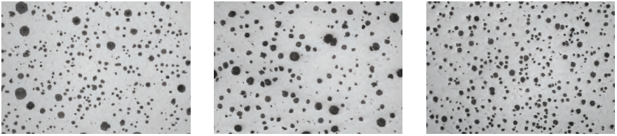
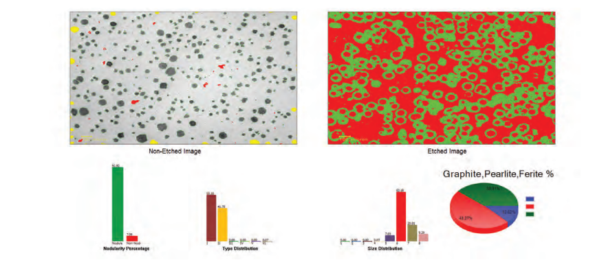
Ductile Iron—also known as Ductile Cast Iron, Nodular Cast Iron, Spheroidal Graphite Iron, or SG Iron—is a graphite-rich type of cast iron. The software uses advanced image processing techniques such as global thresholding, boundary detection, and artificial neural networks for analysis.
Nodules that touch image boundaries are excluded, and artifacts smaller than 10 microns are filtered out. Nodules and non-nodules are classified based on predefined spheroidicity.
During analysis, the software computes key quality parameters including:
- Nodule Count
- Nodule Size (classified by Arabic numerals 1 to 8)
- Nodule Form (classified by Roman numerals I to VI)
All measurements are performed automatically with a single button click.
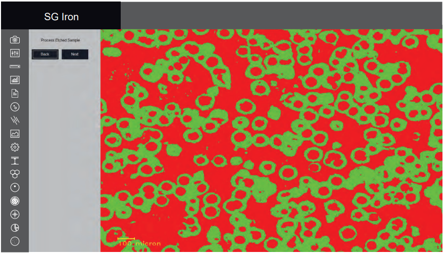
In the second step, etched samples are analyzed. The software automatically calculates the percentage of Graphite and Pearlite present. Results from both non-etched and etched samples are compiled directly into a spreadsheet within the image analysis interface.
Comprehensive reports—including all relevant data and associated images—are generated instantly with one click.
Ductile Iron/Nodularity
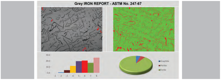
Gray Iron/Graphite Flakes
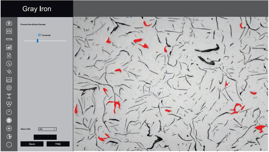
Gray Iron, or Gray Cast Iron, is characterized by a graphite flake structure formed during the cooling process. It is named for the gray appearance of its fracture surface, caused by the presence of graphite.
This module automatically measures the length of graphite flakes in gray iron samples. Shorter Type A graphite flakes indicate higher strength and improved ductility. With a single click, the software quantitatively analyzes graphite length through metallographic imaging.
Graphite sizes are reported across eight classes (1–8), in accordance with ASTM A247-67 or ISO 945-1 standards. The software also categorizes graphite flakes into types A, B, C, D, and E, based on their orientation within the microstructure.
In etched samples, the software calculates the percentage of pearlite by excluding the graphite area. The matrix composition—including pearlite, ferrite, and graphite—is then reported.
Comprehensive reports are generated automatically, aligned with the international standards selected by the user.
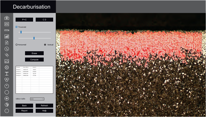
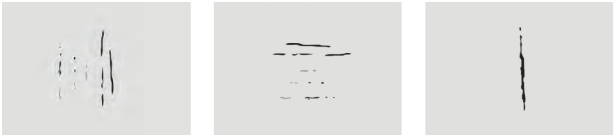
Decarburization
This module is used to determine the depth of decarburization based on changes in the material's microstructure. Partial decarburization refers to a reduction in carbon content without complete loss. The software measures decarburization depth in the workpiece up to the boundary of the ferritic layer, where nearly all carbon has been removed.
All measurements are performed in compliance with ASTM E1077-91 standards.
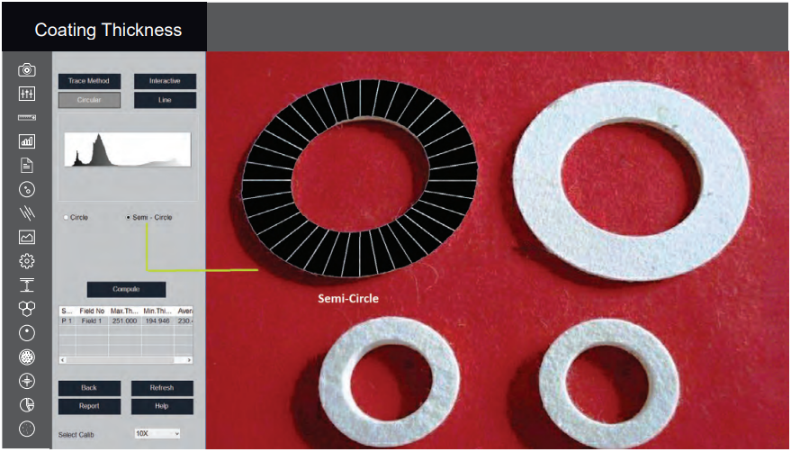
Coating Thickness
Plating or coating thickness is measured using a cross-sectional microscopy method. The specimen is sectioned, mounted, polished, and then examined under an optical microscope. In some cases, etching the base metal may be required to clearly distinguish the coating layer and ensure accurate measurement.
This method is used to evaluate the local thickness of metal and oxide coatings through microscopic examination of cross-sections. Under optimal conditions, the optical microscope can achieve a measurement accuracy of up to 0.8 microns. This level of precision makes the method well-suited for evaluating thin coatings.
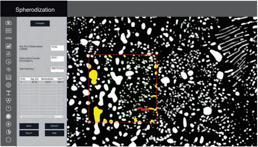
Spherodization
This module is designed to analyze spheroidal graphite (nodules) in cast iron samples. Nodules are distinguished from non-nodules based on predefined spheroidicity criteria. In the visual output, nodules are highlighted in blue, while non-nodules appear in red.
Each nodule is classified by form (designated by Roman numerals I to VI) and size (designated by Arabic numerals 1 to 8). The module also calculates and reports the number of nodules per square millimeter (nodules/mm²).
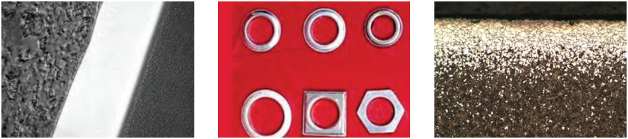
Carbide Banding
Iron carbide, also known as cementite, is an intermetallic compound of iron and carbon. It is commonly found in steels and cast iron. Additionally, iron carbide can be produced as a raw material through the iron carbide process, which is part of a group of alternative iron-making technologies.

Non Metallic Inclusion
MaterialQ+™ software allows users to identify four types of non-metallic inclusions in metallographic samples:
- Sulfide Type (Type A)
- Alumina Type (Type B)
- Silicate Type (Type C)
- Globular Type (Type D)
Each inclusion type is further categorized as Thin or Heavy, based on their width characteristics.

Settings
The Settings module is used to configure essential parameters during the initial software setup. Options include selecting ISO/ASTM calibration standards, customizing the report format, and defining which parameters appear on printed report images.
Once the settings are configured, a single click enables all analyses using the saved preferences. These settings are stored permanently and do not need to be changed routinely unless specific updates or changes in requirements occur.

Clicking the Settings icon opens a new interface that helps streamline your workflow. By selecting the correct options through radio buttons, you reduce the chance of error and enable one-click operation throughout the software.
1. Report Type
Choose the preferred report format—ASTM or ISO. Once selected, it will remain the default until you choose to modify it.
2. Set Default Workflow
Select how you prefer to work:
- Live Display – Analyze images in real-time.
- Stored Images – Capture all images first and analyze them later.
3. Select Calibration
Choose from pre-stored calibration data. Most Cast Iron analysis is typically done using the 100X objective.
4. Set 100 Micron Scale Bar
Choose whether to display a scale bar on images:
- Enable "Show Boundary" to display contours around graphite.
- Enable "Show Number" to display count labels on graphite features.
5. Set Gallery Path
The gallery path is preset, but you may update it if needed.
6. SG Iron Options
Several display options are available for SG Iron analysis. You can choose to show or hide specific parameters. If no selection is made, a default contour will be created.
7. Aspect Ratio
This setting is typically fixed. Modify only if specifically required.
8. Report Template Options
Two report formats are available:
- With chemical composition and physical property data
- Without chemical and physical data
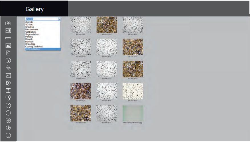
Gallery
The software provides quick access to captured images through organized folders. The following folders are available:
- Measurement
- Segmentation
- Grain Size
- Porosity
- Decarburization
- SG Iron
- Gray Iron
Each folder helps you easily locate and review images related to specific analysis types.
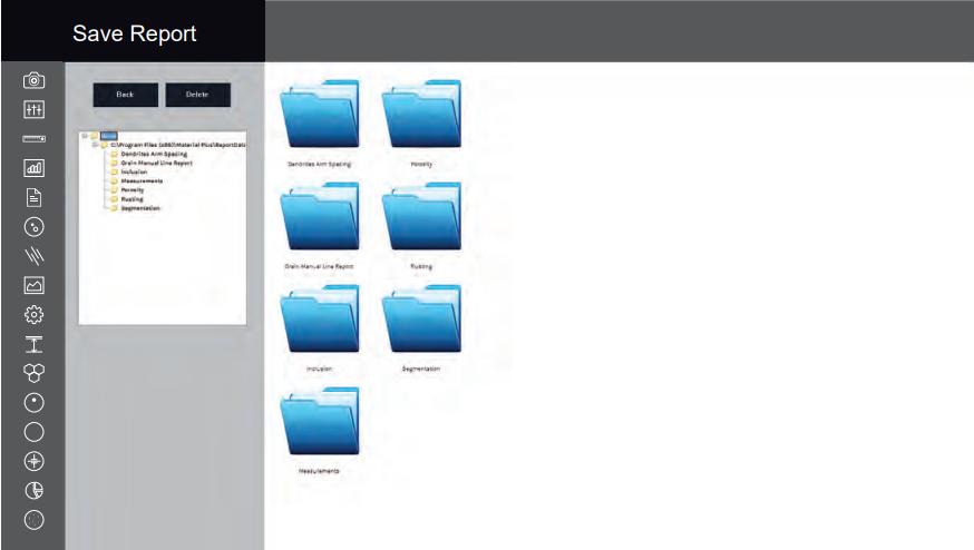
Save Report
All reports are saved in a folder and can be retrieved at any time in the future.