Principle of X-ray Fluorescence Analysis
Characteristic X-Rays of Elements
Different elements have extra-nuclear electronic orbitals with varying binding energies. As a result, when excited, they emit X-ray photons with distinct energies. Each element emits X-rays at its unique energy, representing its characteristic signature, thus termed as characteristic X-rays. The characteristic X-ray of each element has a specific wavelength. By detecting X-rays of these specific wavelengths, we can identify the presence of the target element in a sample.

Principle of Wavelength Dispersive Spectroscopy
When many elements coexist in a sample and are irradiated by primary X-rays from the X-ray tube, they emit their corresponding characteristic X-rays, generally known as X-ray fluorescence. The process of separating and measuring these characteristic X-rays is called X-ray Fluorescence Spectroscopy.
Since the characteristic X-rays of different elements have specific wavelengths, they can be separated using Crystal Diffraction based on Bragg's Equation. This type of spectroscopy is known as Wavelength Dispersive Spectroscopy.
Bragg's Law:
nλ=2dsinθ
In this equation:
- d is the distance between atomic layers in a crystal.
- θ is the angle of incidence.
- λ is the wavelength of the incident X-ray.
- nis an integer representing the order of diffraction.
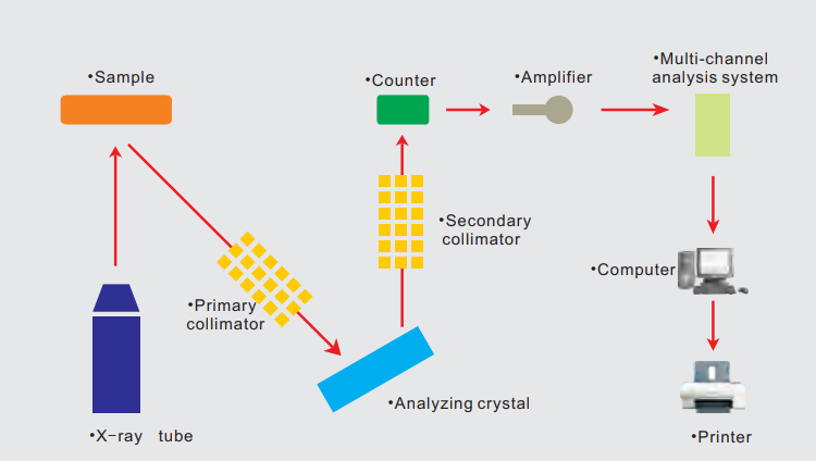
Working Principle of Wavelength Dispersive Spectrometer
Software Overview
Software Functions:

Technical Specifications:
Self-developed software system for the X-ray Fluorescence Analyzer, compatible with Windows operating systems. The system features an easy-to-use interface entirely in Chinese.
Using innovative full-spectrum analysis technology, it allows for real-time tracing and correction of every spectrum line. This significantly enhances the repeatability and stability of quantitative analysis and provides clear evidence for diagnosing instrument status.
The software includes two quantitative analysis algorithms: the empirical coefficient algorithm and the theoretical a-coefficient algorithm. The latter reduces the number of standard samples required while maintaining high accuracy.
It supports analysis data processing, linear fitting, and various matrix corrections. Characteristic values can be calculated based on analysis results. User interaction is facilitated for setting and modifying parameters, ensuring timely output of analysis data and reports. Comprehensive self-diagnosis measures are also included.
Wavelength dispersive instrument spectrum
Examples of Cement Industry
Cement standard XS04-2
| XS04-2 | Si | Al | Fe | Ca | Mg |
| Standard value | 12.71 | 2.86 | 3.09 | 43.29 | 1.6 |
| Average Value | 12.708 | 2.912 | 3.056 | 43.305 | 1.635 |
| Max value | 12.74 | 2.93 | 3.06 | 43.34 | 1.66 |
| Min value | 12.69 | 2.89 | 3.05 | 43.30 | 1.62 |
| Range | 0.05 | 0.04 | 0.01 | 0.04 | 0.04 |
| Standard deviation value | 0.015362 | 0.01077 | 0.004899 | 0.01145 | 0.014318 |
| Relative deviation value(%) | 0.120887 | 0.36986 | 0.160307 | 0.02644 | 0.875708 |
Cement standard XS05-2
| XS05-2 | Si | Fe | Al | Ca | K | Na | Mg |
| Standard value | 12.71 | 3.09 | 2.86 | 43.29 | 0.45 | 0.28 | 1.6 |
| Average value | 12.706 | 3.091 | 2.903 | 43.273 | 0.454 | 0.295 | 1.62 |
| Max value | 12.73 | 3.1 | 2.92 | 43.3 | 0.46 | 0.35 | 1.64 |
| Min value | 12.69 | 3.08 | 2.88 | 43.25 | 0.45 | 0.27 | 1.6 |
| Range | 0.04 | 0.02 | 0.04 | 0.05 | 0.01 | 0.08 | 0.04 |
| Standard deviation value | 0.012806 | 0.008307 | 0.011 | 0.015524 | 0.004899 | 0.02377 | 0.013416 |
| Relative deviation value(%) | 0.100789 | 0.268736 | 0.378918 | 0.035875 | 1.07907 | 8.057535 | 0.828173 |
Examples of Steel Industry:
Results of Agglomerate Measurement
Below are the results of repeated tests of the unknown sample:
| No. | Sample No. | Measurement Time | Fe(%) | CaO(%) | MgO(%) | SiO2(%) | So3(%) |
| 1 | 17# | 2007-11-09 13:35 | 53.87 | 12.10 | 3.44 | 5.73 | 0.040 |
| 2 | 17# | 2007-11-09 13:39 | 53.89 | 12.08 | 3.43 | 5.74 | 0.040 |
| 3 | 17# | 2007-11-09 13:42 | 53.91 | 12.08 | 3.44 | 5.75 | 0.039 |
| 4 | 17# | 2007-11-09 13:46 | 53.91 | 12.10 | 3.44 | 5.76 | 0.040 |
| 5 | 17# | 2007-11-09 13:50 | 53.90 | 12.07 | 3.45 | 5.76 | 0.039 |
| 6 | 17# | 2007-11-09 13:53 | 53.89 | 12.09 | 3.43 | 5.75 | 0.041 |
| 7 | 17# | 2007-11-09 13:57 | 53.90 | 12.09 | 3.45 | 5.75 | 0.042 |
| 8 | 17# | 2007-11-09 14:01 | 53.89 | 12.09 | 3.46 | 5.76 | 0.040 |
| 9 | 17# | 2007-11-09 14:05 | 53.89 | 12.09 | 3.44 | 5.75 | 0.039 |
| 10 | 17# | 2007-11-09 14:08 | 53.88 | 12.08 | 3.44 | 5.75 | 0.040 |
Test of 18-hour stability taken by unknown sample 17#; the results after total 306 times are:
| Constituent | Average value | Min value | Min value | Standard deviation value |
| Fe(%) | 53.891 | 53.850 | 53.920 | 0.012 |
| CaO(%) | 12.086 | 12.040 | 12.120 | 0.014 |
| MgO(%) | 3.446 | 3.420 | 3.470 | 0.010 |
| SiO2(%) | 5.752 | 5.710 | 5.780 | 0.010 |
| So3(%) | 0.040 | 0.038 | 0.042 | 0.001 |
Converter slag
Below are the results of repeated tests of the unknown sample:
| No. | Sample No. | Measurement Time | Fe(%) | SiO2(%) | CaO(%) | MgO(%) |
| 1 | D1-2702A | 2007-11-12 16:52 | 12.75 | 7.74 | 50.41 | 9.11 |
| 2 | D1-2702A | 2007-11-12 16:56 | 12.73 | 7.75 | 50.39 | 9.12 |
| 3 | D1-2702A | 2007-11-12 17:00 | 12.71 | 7.77 | 50.38 | 9.14 |
| 4 | D1-2702A | 2007-11-12 17:04 | 12.73 | 7.78 | 50.35 | 9.14 |
| 5 | D1-2702A | 2007-11-12 17:08 | 12.74 | 7.78 | 50.33 | 9.15 |
| 6 | D1-2702A | 2007-11-12 17:11 | 12.76 | 7.80 | 50.27 | 9.18 |
| 7 | D1-2702A | 2007-11-12 17:15 | 12.76 | 7.80 | 50.27 | 9.18 |
| 8 | D1-2702A | 2007-11-12 17:19 | 12.76 | 7.80 | 50.25 | 9.18 |
| 9 | D1-2702A | 2007-11-12 17:22 | 12.77 | 7.81 | 50.24 | 9.19 |
| 10 | D1-2702A | 2007-11-12 17:26 | 12.76 | 7.82 | 50.24 | 9.23 |
Test of 15-hour stability taken by unknown sample D1-2702A#; the results after total 253 times are:
| Constituent | Average value | Min value | Max value | Standard deviation value |
| Fe(%) | 12.782 | 12.710 | 12.840 | 0.021 |
| SiO2(%) | 7.818 | 7.740 | 7.840 | 0.011 |
| CaO(%) | 50.215 | 50.160 | 50.410 | 0.030 |
| MgO(%) | 9.217 | 9.110 | 9.290 | 0.027 |
